Seldom data is present just in the form needed by an optimization algorithm. Most of the time a preprocessing of input data (conversion, aggregation, formatting) is necessary.
After the optimization, the results must be postprocessed and displayed graphically.
Mathematica offers for this purpose an optimal platform with all required functionality.
Because Mathematica is an interactive and interpreting environment, the user gets ongoing intermediate results and is able to decide for the most promissing steps to get a solution.
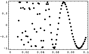
An example might serve as clarification. The values are printed in an abbreviated form, the plot shows all values.
data = {{0.01, -0.506366}, {0.011, 0.195822}, ..., {0.029, 0.0746909}, {0.03, 0.94053}, {0.031, 0.746068}, ..., {0.1, -0.544021}}
ListPlot[data, Frame -> True, Axes -> False, PlotStyle -> PointSize[0.02]]

It is numerically difficult to obtain the slope at x-position 0.03. Easier is a symbolic derivative of a fit of the data.
fit = Fit[data, {1, Sin[x], Sin[1/x]}, x]
8.38*^-16 + 1.*Sin[1/x] - 1.4*^-14*Sin[x]
fit = Chop[fit]/.{1.0->1}
Sin[1/x]
deriv = D[fit, x]
-Cos[1/x]/x^2
Inserting the explicit x-value yields the desired result:
deriv/.x->0.03
377.458